The GIS of the GMSA was structured in ArcGIS 10.2.2 software. For this, a File Geodatabase was created with the following datasets: Base Map, Sources, Geology, Oceanic Structures, and Tectonic Plates. Each of these datasets is made up of related entities or feature classes; for example, Geology comprises the feature classes of chronostratigraphic units, faults, folds, basic dikes, volcanic and intrusive alkaline‒carbonatites, blueschists and eclogites, kimberlite fields, impact craters, Quaternary volcanoes, and their annotations, which identify these entities on the map. The structure of the GIS of the GMSA is illustrated in Figure 8.
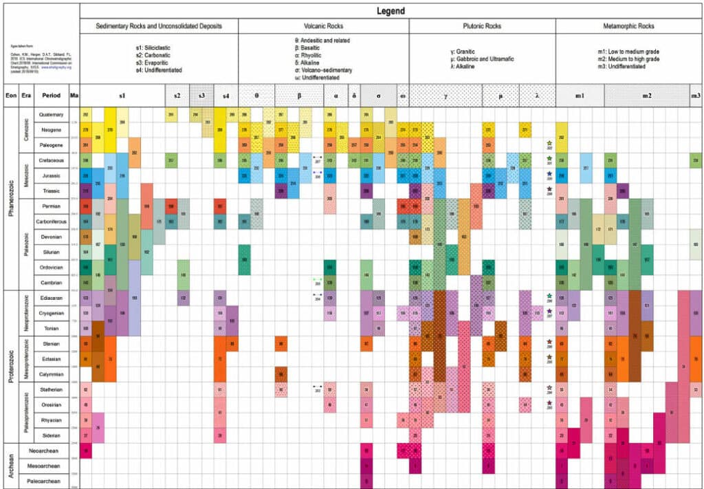
18 to Neoarchean volcano–sedimentary rocks (2800–2500 Ma).
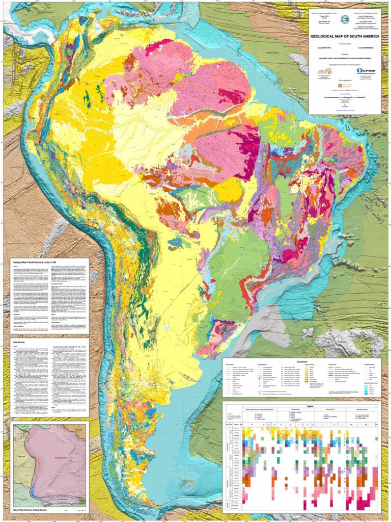
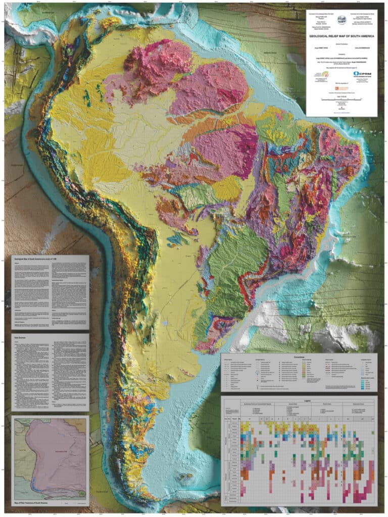
The inset Map of Plate Tectonics of South America shows the locations and boundaries of the plates associated with the continent and its tectonic framework: South American, Nazca, Cocos, Caribbean, Antartic, Scotia, Sandwich, and African. In addition, the distribution of Quaternary volcanoes is shown, while the Andean deformation belt is differentiated from the South American platform.
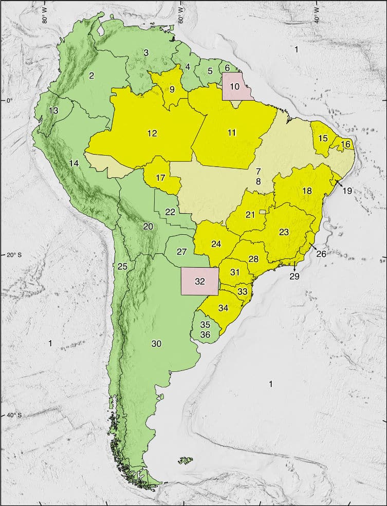
Another inset indicates all the geological maps that were used in the compilation of the GMSA, illustrated in Figure 3.
Geographical Information Systems (GIS)
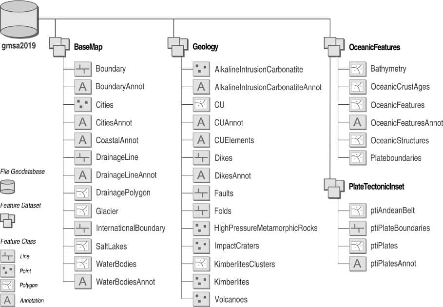
The GIS of the GMSA was structured in ArcGIS 10.2.2 software. For this, a File Geodatabase was created with the following datasets: Base Map, Sources, Geology, Oceanic Structures, and Tectonic Plates. Each of these datasets is made up of related entities or feature classes; for example, Geology comprises the feature classes of chronostratigraphic units, faults, folds, basic dikes, volcanic and intrusive alkaline‒carbonatites, blueschists and eclogites, kimberlite fields, impact craters, Quaternary volcanoes, and their annotations, which identify these entities on the map. The structure of the GIS of the GMSA is illustrated in Figure 8.
Figure 8. Structure of the Geographical information system of the GMSA in ArcGIS.
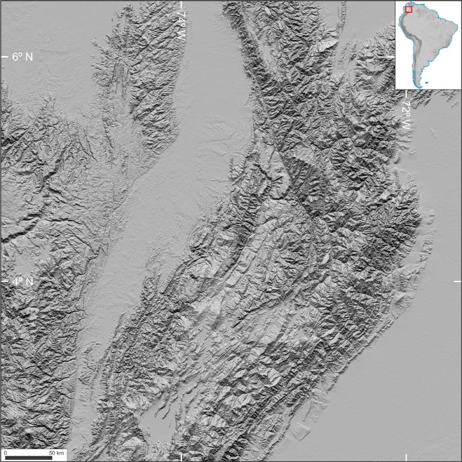
The GMSA has a scale of 1:5,000,000, follows the WGS–1984 coordinate system, and its graphical output has a polyconic projection with a latitude of origin at the Equator and longitudinal origin at the central meridian of 59° west of Greenwich.
The GMSA was released to the public on November 26, 2019, in GIS (MXD, style, File Geodatabase), high–resolution PDF (print version), low–resolution PDF (web), TIFF, and fonts, allowing recreation of the CU patterns. Additionally, the web service and ArcGIS Online were implemented; the latter can be easily deployed on a mobile device (Figure 9).